
In data science, one of the challenges we try to address consists on fitting models to data. The objective is to determine the optimum parameters that can best describe the data. For example, if we have the following linear model:
we want to determine the optimum β's which best fits the observed values of y.
A challenge that we face is that the range of the values for X can be different. For example, X1 and X2 can range from 0 - 1 and 0 - 1e20, respectively. Therefore, the algorithms that try to extract the β's will perform poorly.
In this post we will demonstrate the challenges presented when the ranges of each feature are different, and how to address them by applying a normalization (scaling) technique.
CREATING THE DATA SET
We start by creating three data sets with one feature (X) as plotted below. The range of X is 0 - 1e-20, 0 - 1 and 0 - 1e20 for the "Low", "Medium" and "High" data sets, respectively. The y-values have the same range across all three data sets. The Python code and the figures that display the data are presented below.
X_med = np.linspace(0,1,1001)
X_high = 1e20*X_med
X_low = 1e-20*X_med
y_real = np.cos(2/3*2*np.pi*X_med-np.pi/8)
y = y_real + (np.random.randn(len(X_med)))/5 # add some noise
Figure 1: Data and Ground Truth for three different ranges of X.
It can be observed that although the X-axis is different for each data set, the y-axis is the same.
FITTING A LINEAR REGRESSION MODEL
We will use a linear regression model to fit the data to the only feature we have X. The model is described by:
def fit_model_1(X, y):
    if len(X.shape)==1:
        X2 = X.reshape(-1,1)
    else:
        X2 = X
    reg = linear_model.LinearRegression(fit_intercept=False)
    reg.fit(X2,y)
    y_pred = reg.predict(X2)
    return y_pred
In the figure below we notice that the model fitted to the data for all three ranges.

Figure 2: Data, Ground Truth and Model to a simple linear fit for three different ranges of X.
MAKING POLYNOMIALS
We observe that the model is very similar regardless of the range of X. However, a straight line is not a good model to fit to this data set. To improve the model we can add complexity by creating more features using a 3rd order polynomial. The new model will have the following form:
Therefore, for every data point Xi, we will have a new vector Xi' given by:
The vector will have a length of 4 because it includes the bias (intercept) term 1.
def make_poly(deg, X, bias=True):
p = PolynomialFeatures(deg,include_bias=bias) # adds the intercept column
X = X.reshape(-1,1)
X_poly = p.fit_transform(X)
return X_poly
We now apply a linear regression to the polynomial features, and obtain the results of the model presented below.

Figure 3: Third order polynomial fit of a linear regression model to three different ranges of X without normalization.
In the figure above, we appreciate that the model is very different for each range of X. We note that the "Medium" range tends to fit the model well, while the "Low" and "High" range do a poor job. This occurs because the range for every feature (polynomial value) is very different for the "Low" and "High" range, but it is similar (or the same) for the "Medium" range.
In the table below, we present the maximum value for each of the features in the "Low", "Medium" and "High" range after expanding it to a 3rd order polynomial. For the "Medium" range, the maximum value for all features is 1. However, for the "Low" and "High" range, the maximum value of the features varies from 1e-60 to 1 and 1 to 1e60, respectively.
The maximum value for each feature is:
Range Bias X X^2 X^3
____________________
Low 1 1e-20 1e-40 1e-60
Medium 1 1 1 1
High 1 1e20 1e40 1e60
The algorithms that find the best β's do not perform well when the maximum value for each feature has different orders of magnitude.
FEATURE SCALING
To address this we can scale (normalize) the data. Although there are several ways of normalizing the data, we will use a method for which we subtract the mean and divide by the standard deviation, as presented below:
def normalize(X_poly):
# remove the bias column which should not be normalized!
X_poly_2 = np.delete(X_poly, np.s_[0], 1)
# scale each column
scaler = StandardScaler()
X_poly_3 = scaler.fit_transform(X_poly_2)
# re-add the bias term
ones = np.ones((len(X_poly_3),1))
X_poly_4 = np.append(ones, X_poly_3, 1)
return X_poly_4
The maximum value for each feature after normalization is:
Range Bias X X^2 X^3
___________________
Low 1 1.7 2.2 2.6
Medium 1 1.7 2.2 2.6
High 1 1.7 2.2 2.6
We observe that after normalization, the maximum value for each feature is in the same order of magnitude, and the results are good fits for the "Low", "Medium" and "High" range feature of X.
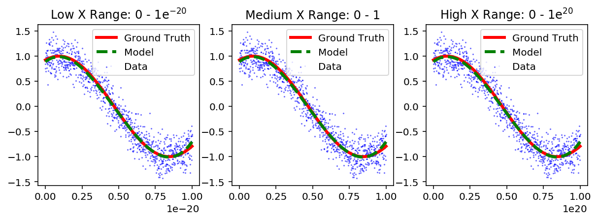
Figure 4: Third order polynomial fit of a linear regression model to three different ranges of X with normalization.
After scaling the features we get an accurate prediction for the y-axis. In summary, the algorithms used to find the optimum β's that best fit the data work better when the range of the features is within the same order of magnitude.
The code used in this post can be found here.