
This is part 2 of a post where we demonstrate how to plot functions in Tableau. Part 1 can be seen here.
In this section we are focused on using Polar coordinates. This is a helpful system for recreating shapes that have some sort of circular shape. In Cartesian coordinates, each point is represented by an (x,y) pair; however, in the Polar coordinates, each point is represented by a (r,θ) pair.
A few things to keep in mind about angles (θ).
A circle has 360 degrees, which is also known as 2π radians
θ(degrees) = θ(radians)*180/π
Similarly, as in the previous post, we only need two pieces of information, (a) a data file, and (b) the equations we want to use.
Here, we are going to focus on five shapes that demonstrate different designs we can plot with Polar coordinates. The shapes we will analyze are: circles, incomplete circles and hearts, spirals and stars (we are using the word “stars” loosely to encapsulate a variety of shapes). These are shown below.

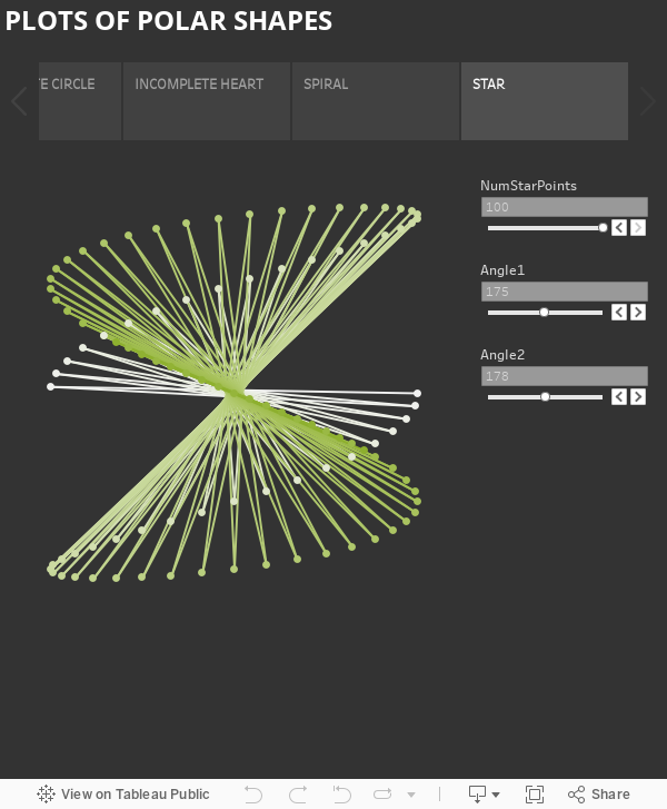
In the figure above we have (A) a circle, (B) an 85% complete circle, (C) an 85% complete heart, (D) a spiral with 5 loops, (E) a star (NumStartPoints = 7, Angle1 = 60, Angle2 = 60), (F) a star (NumStartPoints = 20, Angle1 = 145, Angle2 = 145), (G) a star (NumStartPoints = 73, Angle1 = 65, Angle2 = 65), (H) a star (NumStartPoints = 73, Angle1 = 145, Angle2 = 145), (I) a star (NumStartPoints = 51, Angle1 = 258, Angle2 = 131), (J) a star (NumStartPoints = 100, Angle1 = 175, Angle2 = 178), (K) a star (NumStartPoints = 91, Angle1 = 28, Angle2 = 84), (L) a star (NumStartPoints = 91, Angle1 = 76, Angle2 = 120).
A. DATA
The data file requires a minimum of one column and two rows.

B. CIRCLE
In our first example we will recreate a circle chart.
B.1 RADIUS PARAMETER
We will define a parameter for the radius of the circle.

B.2 POINTS IN θ
We will define an array that has all the values in θ where we want to draw a point.
To obtain this, we will use a method referred to as “densification”.
B.2.1 θ DENSIFICATION
We create an array that has a length equal to the number of points we want to draw in the edge of the shape.
We create a calculated field (RangeEnds) where we assign a datapoint a value of 0, and the other datapoint a value of 1. This defines the ends, such that we can fill in between the number of points we want to obtain.

We will create bins from the RangeEnds using a Size of bins of 0.01, which provides 101 points.

Next, we create an Index calculated field:

B.2.2 θ ARRAY
We create the arrays that have all the values in θ where we want to draw a point. The array will have values between 0 and 2π.

B.3 X AND Y LOCATIONS
Here we calculate the X and Y locations of each point using:


B.4 VISUALIZING THE CIRCLE
To visualize the circle, we will:
Drag RangeEnds (bin) to Rows. Make sure the “Show Missing Values” is checked!
Drag RangeEnds (bin) from Rows to Detail.
Drag X_Circle to Columns, and Y_Circle to Rows. “Compute Using” RangeEnds (bin).
Format and have fun!
C. INCOMPLETE CIRCLE AND HEART
The next example we will recreate an incomplete circle and heart chart.
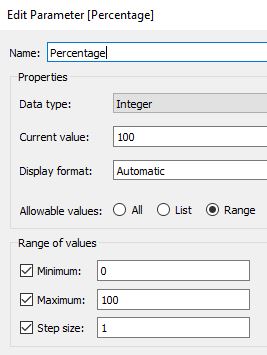
C.1 PERCENTAGE PARAMETER
We will define a parameter called Percentage that informs how complete the shape is. For example, when Percentage is 100%, the shape will be completely drawn, and when Percentage is 75%, only ¾ of the shape will be drawn.
C.2 POINTS IN θ
Here we will use the same data created in section B.2 above.
We will expand this by creating a new Calculated Field called ThetaIncomplete, which will have the ThetaCircle values where we want to draw a point, and NULL otherwise.

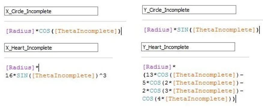
C.3 X AND Y LOCATIONS
Here we calculate the X and Y locations of each point. For the incomplete circle we use the same equations as the circle (shown above), but we replace ThetaCircle with ThetaIncomplete. For the heart we are going to use the heart equations given by:

C.4 VISUALIZING THE INCOMPLETE CIRCLE AND HEART
To visualize the incomplete shapes, we will:
Drag RangeEnds (bin) to Rows. Make sure the “Show Missing Values” is checked!
Drag RangeEnds (bin) from Rows to Detail.
For circle: Drag X_Circle_Incomplete to Rows, and Y_Circle_Incomplete to Columns. “Compute Using” RangeEnds (bin).
For heart: Drag X_Heart_Incomplete to Columns, and Y_Heart_Incomplete to Rows. “Compute Using” RangeEnds (bin).
Change Marks to Line.
Drag Index to Path.
Format and have fun!
D. SPIRAL
The next example we will plot a spiral chart.
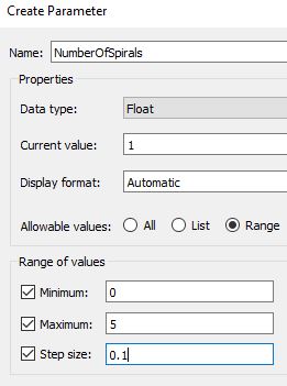
D.1 NUMBER OF SPIRALS PARAMETER
We will define a parameter called NumberOfSpirals that informs how many circles will be in the spiral.
D.2 POINTS IN θ
Here we will use the same data created in section B.2 above.
We will expand this by creating a new calculated field called ThetaSpiral, which will have values that can go beyond 2π when there is more than one circle.

D.3 X AND Y LOCATIONS
We calculate the X and Y locations of each point using.

D.4 VISUALIZING THE SPIRAL
To visualize the incomplete shapes, we will:
Drag RangeEnds (bin) to Rows. Make sure the “Show Missing Values” is checked!
Drag RangeEnds (bin) from Rows to Detail.
Drag X_Spiral to Columns, and Y_Spiral to Rows. “Compute Using” RangeEnds (bin).
Format and have fun!
E. STAR
In our final example, we will plot a star chart.
E.1 NUMBER OF STAR POINTS AND ANGLE PARAMETERS
We will define 3 parameters for the star, the number of points (NumStarPoints), and two angle parameters (Angle1 and Angle2).

E.2 POINTS IN θ
We will define an array that has all the values in θ where we want to draw a point.
E.2.1 θ DENSIFICATION
We create an array that has a length equal to the number of points we want to draw in the edge of the shape.
We create a calculated field (RangeEndsStar) where we assign a datapoint a value of 0, and the other datapoint a value of (NumStarPoint-1)*0.01. This defines the ends, such that we can fill in between the number of points we want to obtain.

We will create bins from the RangeEndsStar using a Size of bins of 0.01.

E.3 X AND Y LOCATIONS
Here we calculate the X and Y locations of each point using:

E.4 VISUALIZING THE STAR
To visualize the star, we will:
Drag RangeEndsStar (bin) to Rows. Make sure the “Show Missing Values” is checked!
Drag RangeEndsStar (bin) from Rows to Detail.
Drag X_Star to Columns, and Y_Star to Rows. “Compute Using” RangeEndsStar (bin).
Change Marks to Line.
Drag Index to Path.
Format and have fun!
When Angle1 and Angle2 are the same we can see star shapes; when they differ we observe interesting patterns.
You can play with the different shapes and parameters below.
This concludes the two-part post on plotting functions in Tableau. I also suggest reviewing other great posts by Jeffrey Shaffer and Ken Flerlage.