In this post, we will demonstrate a method for plotting two-dimensional functions in Tableau. We will present examples in both Cartesian and Polar coordinates. This post focuses on the Cartesian system and the follow-up post focuses on the Polar Coordinate system.
Our goal is to demonstrate how to plot functions as the ones shown below:

Let’s start by reviewing a few definitions.
2D Cartesian Coordinates, is a system where every point on a plane is defined by a pair of values in two perpendicular directions. We commonly call them the X and Y axis.
2D Polar Coordinates, is a system where every point on a plane is defined by a pair of values provided by a distance from a reference point (known as a radius “r”) and an angle (θ).
Why do we have two different coordinates systems?
The reason we have two coordinate systems (actually, there are a lot more than two), is that sometimes it is easier to solve the mathematical equations in one system over the other. That said, you can switch between systems using transformation equations. For example, if you have x and y in the Cartesian system, you can switch to the Polar by:

Similarly, if we have r and θ in the Polar system, we can switch to Cartesian with:


Now that we have covered the basics let’s dive right in. We only require two pieces of information, (a) a data file, and (b) the equations we want to use.
A. DATA
For data, we should have a file with as little as one column and two rows.

B. POINTS IN THE X-AXIS
We will define an array that has all the values in the X-axis where we want to draw a point. To obtain this, we will use a method referred to as “densification”.
B.1 X-AXIS DENSIFICATION
We create an array that has a length equal to the number of points we want to draw in the X-direction. We could obtain this from the original data file, which would simplify things. However, if we do not have this information in the main data file, we create our own. We generate a calculated field (RangeEnds) where we assign one of the datapoints a value of 0, and the other datapoint a value of 1. This defines the ends, such that we can fill in between the number of points we want to obtain.

We select the number of points (N) that we want, and we create a bin from the RangeEnds with a Size of bins equal to 1/(N-1). Therefore, if we want 11, 101, and 1001 points, we would use a Size of bins of 0.1, 0.01, and 0.001, respectively.

Next, we create an Index calculated field:

Why do we have an Index if we already have the RangeEnds (bin)? Aren’t they equivalent?
They are technically similar. We will use these values inside other calculated fields, and Tableau does not allow “results of type numerical bin” in the calculated fields, so the workaround is to use the Index.

B.2 X-AXIS ARRAY
Next, we define the range for the X-axis. We can use any values such as -7 to 7, 3 to 20, -10 to -5.2, etc.
We create two parameters that define the minimum and maximum X-value.
We then create a custom field called X-Cart which will have the locations in the X-axis for the datapoints.

X-Cart has N values equally distributed between X-Min and X-Max.
C. POINTS IN THE Y-AXIS
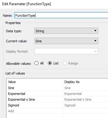
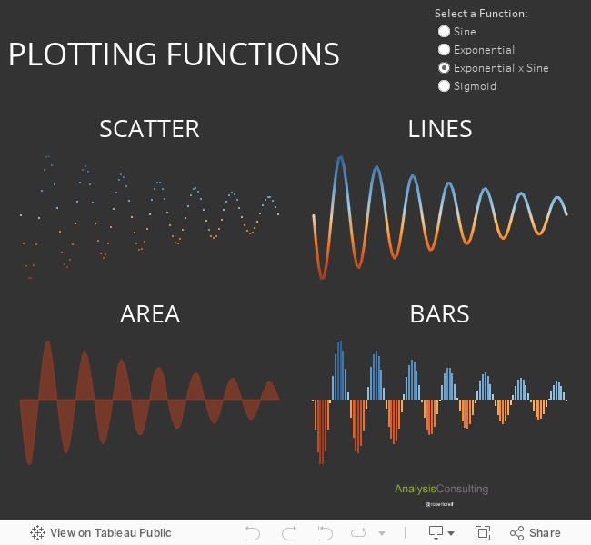
Now that we have the X-axis defined, we define the location of the points in the Y-axis. For this we need the equation that extracts a Y-value as a function of the X-value. We will create four examples: a sine wave, an exponential, an exponential * sine, and a sigmoid (usually used for Sankey diagrams).
We produce a parameter that allows us to select the FunctionType.
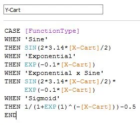
We create a calculated field (Y-Cart) which has the equations of the four examples we want to use. We use a Case function that depends on the FunctionType parameter.
D. VISUALIZING
For this example, we are using Size of bins = 0.01, X-Min = -7 and X-Max = 7.
Drag Range Ends (bin) to Rows. Make sure the “Show Missing Values” is checked!
Drag Range Ends (bin) from Rows to Detail.
Drag X-Cart to Column, and “Compute Using” Range Ends (bin).
Drag Y-Cart to Row, and “Compute Using” Range Ends (bin).
Format as you wish!
Below are the results we obtained.
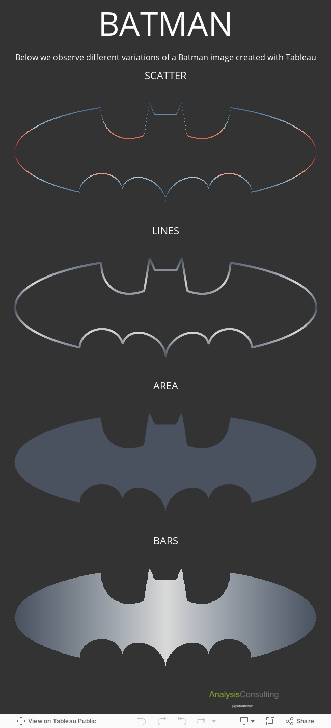
E. HAVING FUN (‘BATMAN’)
We do not have to limit our plots to simple sine waves or exponentials. We can expand to more complicated shapes.
Below, we have drawn the “Batman Curve” .
To do this, we replace step “C” above by creating two calculated fields. One field draws the upper part of the curve (above zero) and the other field draws the lower part (below zero).
The equations for the top curve are the following:

The equations for the bottom curve are the following:


You can copy-paste the equations here:
Y-Top:
IF [X-Cart]<=-3 OR [X-Cart]>=3
THEN 3*sqrt(1-([X-Cart]/7)^2)
ELSEIF abs([X-Cart])>0.75 AND ABS([X-Cart])<1
THEN 9-8*abs([X-Cart])
ELSEIF abs([X-Cart])>0.5 AND ABS([X-Cart])<0.75
THEN 0.75+3*abs([X-Cart])
ELSEIF abs([X-Cart])<0.5
THEN 2.25
ELSEIF abs([X-Cart])>1 AND abs([X-Cart])<3
THEN 6*SQRT(10)/7+
(1.5-0.5*ABS([X-Cart]))-
6*SQRT(10)/14*SQRT(4-(ABS([X-Cart])-1)^2)
END
Y-Bottom:
IF abs([X-Cart])>=4
THEN -3*sqrt(1-([X-Cart]/7)^2)
ELSE
ABS([X-Cart]/2)-
(3*SQRT(33)-7)/112*[X-Cart]^2-
3+
SQRT(1-(ABS(ABS([X-Cart])-2)-1)^2)
END
F. VISUALIZING
For this example, we are using Size of bins = 0.002, X-Min = -7 and X-Max = 7.
Drag Range Ends (bin) to Rows. Make sure the “Show Missing Values” is checked!
Drag Range Ends (bin) from Rows to Detail.
Drag X-Cart to Column, and “Compute Using” Range Ends (bin).
Drag Y-Top to Row, and “Compute Using” Range Ends (bin).
Drag Y-Bottom to Row, and “Compute Using” Range Ends (bin).
Format as you wish!
Below are the results we obtained.