
A typical map is a two-dimensional representation of a three-dimensional sphere. When we draw paths, we know that the shortest distance between two points is a straight line. Nevertheless, the shortest path on the surface of a sphere does not necessarily look like a straight line on a two-dimensional map.
In this post, we explain how to draw paths that connect two locations on a map based on the shortest distance between them using Tableau. We use a concept called great-circle distance, which is the shortest distance between two locations on the surface of a sphere.
We have included the formulas of all the calculated fields at the end of this post so they can be copy-pasted as needed!
A. DATA
The data needs to have the following form:
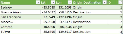
We have a column with the Name of the locations. We have a column for the Latitude and Longitude of each location (*, **). We have a column that defines the origin and destination for each pair of locations. Finally, we have an ID column that indicates the origin-destination pairs. For example, for ID == 1, there is a path between the origin, Sydney (Australia), and the destination, Buenos Aires (Argentina).
B. DRAWING PATHS WITH TWO-DIMENSIONAL STRAIGHT LINES
As a first step, we can quickly create the paths using two-dimensional straight lines. To do this we must make sure we are not aggregating the measure. Then we:
Drag Lon to Column
Drag Lat to Row
Change the Mark to Line
Drag ID to Detail
Drag PathOrder (bin) to Path.
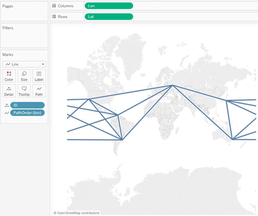
The result is the chart shown above which presents the connections between the cities. However, the connections are simple straight lines in two dimensions, but NOT the shortest paths on a sphere.
For some applications, this chart will suffice. However, if the goal is the shortest path distance, clear your sheet, and continue with the next steps.
C. GREAT CIRCLE EQUATIONS
A great circle is the shortest distance between two locations across the surface of a sphere. I will not go into the details of how to derive the equations. Instead, we present the equations required.

Where Lat_Start and Lon_Start are the latitude and longitude at the origin, and Lat_End and Lon_End are the latitude and longitude at the destination. f is a value that will range between 0 and 1.
D. CALCULATED FIELDS
Here, we present all the fields that require calculations.
D.1. PATH ORDER
We have a field that indicates the path order, in other words, it indicates which is the origin and destination. We will make Origin equal to 0, and Destination equal to 1.

D.2. PATH ORDER DENSIFICATION – PathOrder (bin)
We need a path with a set of points between the start and end locations. Therefore, we generate a data-set that contains the missing values. This process is referred to as “densification”. To do this, we create “Bins” from the PathOrder.
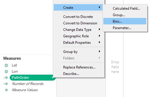
The PathOrder has values of 0 and 1. To define the “Size of the bins”, we first determine how many points we want to use to draw the line. For example, if we want N = 101 points, the "Size of the bins" is given by 1/(N-1) = 1/100 = 0.01.

D.3. LATITUDE AND LONGITUDE START AND END VALUES
We now create the values for the latitude and longitude for the start and end locations.
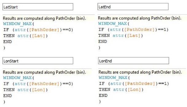
Why do we need these calculations if we already know the values from Lat and Lon?
In the table below we observe that the values of Lat only exist in PathOrder == 0 for the origin, and PathOrder == 1 for the destination. The new calculated fields separate these two values into two different columns (LatStart and LatEnd), and fills in the densified points obtained by the PathOrder (bin). For these fields, “Compute Using” the PathOrder (bin). The same logic applies to Lon.

D.4. GREAT CIRCLE CALCULATIONS
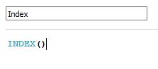
Below we present the calculated fields for d, f, A, B, X, Y, Z, NewLat and NewLong. We will first need an Index field.
d, f, A and B are defined as:
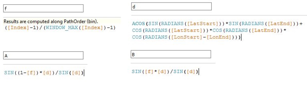
Note that the Lat and Lon values are in degrees, and we require them to be in RADIANS!
X, Y and Z are defined as:

NewLat and NewLon are defined as:

Note that the NewLat and NewLon values are in radians, and we require them to be in DEGREES!
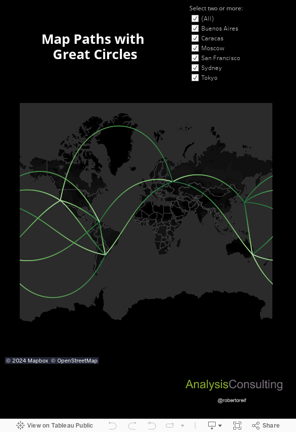
E. VISUALIZING THE MAP PATHS
To visualize the map paths, we must make sure we are not aggregating the measure. Then we need to:
Convert NewLat and NewLon to Geographic Role -> Latitude and Longitude, respectively.
Drag ID to Detail.
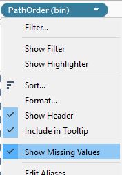
Drag Path Order (bin) to Rows. Make sure the “Show Missing Values” is checked!
Drag the Path Order (bin) from Rows to Details.
Drag NewLon and NewLat to Columns and Rows, respectively; and “Compute Using” PathOrder (bin).
Change the Mark to Line.
Drag PathOrder (bin) to Path.
Format as you wish!
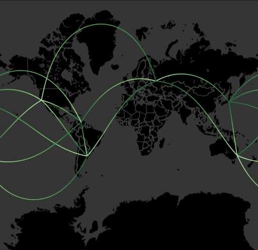
Feel free to play with the map below!
Formulas:
Here, you can copy-paste the formulas into your calculated fields.
d =
ACOS(SIN(RADIANS([LatStart]))*SIN(RADIANS([LatEnd]))+
COS(RADIANS([LatStart]))*COS(RADIANS([LatEnd]))*
COS(RADIANS([LonStart]-[LonEnd])))
f =
([Index]-1)/(WINDOW_MAX([Index])-1)
A =
SIN((1-[f])*[d])/SIN([d])
B =
SIN([f]*[d])/SIN([d])
X =
[A]*COS(RADIANS([LatStart]))*COS(RADIANS([LonStart]))+
[B]*COS(RADIANS([LatEnd]))*COS(RADIANS([LonEnd]))
Y =
[A]*COS(RADIANS([LatStart]))*SIN(RADIANS([LonStart]))+
[B]*COS(RADIANS([LatEnd]))*SIN(RADIANS([LonEnd]))
Z =
[A]*SIN(RADIANS([LatStart]))+
[B]*SIN(RADIANS([LatEnd]))
NewLat =
DEGREES(ATAN2([Z],SQRT([X]^2+[Y]^2)))
NewLon =
DEGREES(ATAN2([Y],[X]))
* Tableau does not allow to drag the generated Latitude and Longitude fields into Calculated Fields; therefore, we need to have these defined in the data.
**West Longitudes need to be written in negative form. For example, Caracas is 10.4806˚N and 66.9036˚W. We would use the values 10.4806 and -66.9036. This does not apply to East Longitudes, nor any of the Latitudes.